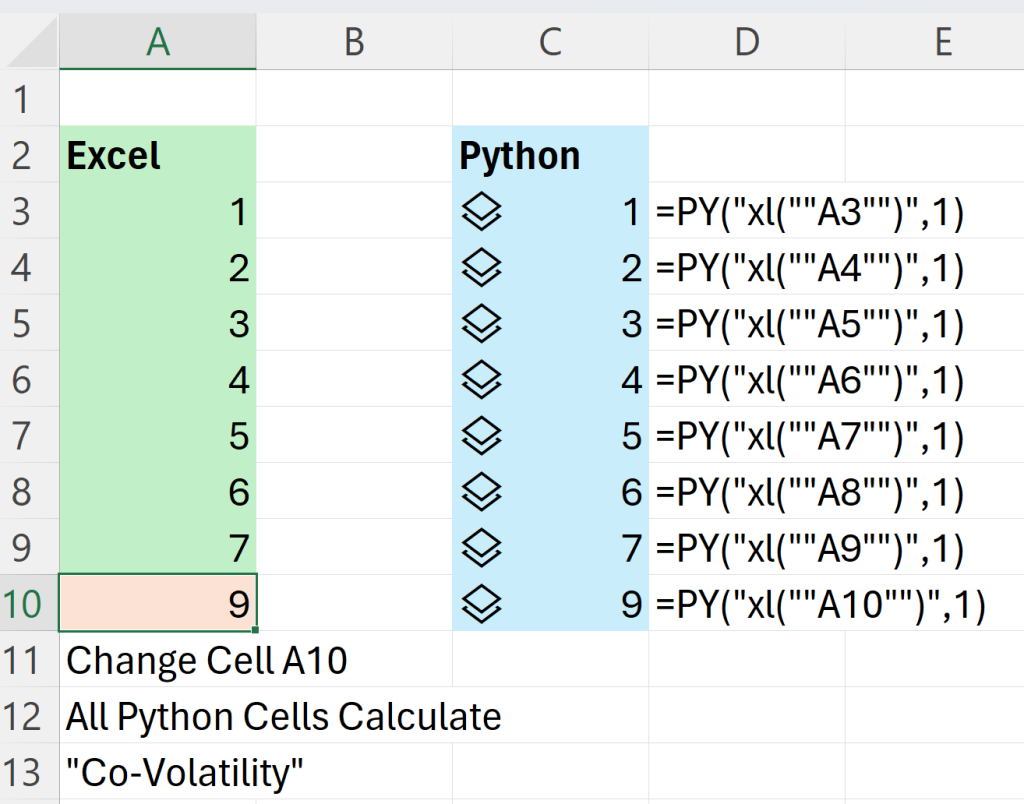
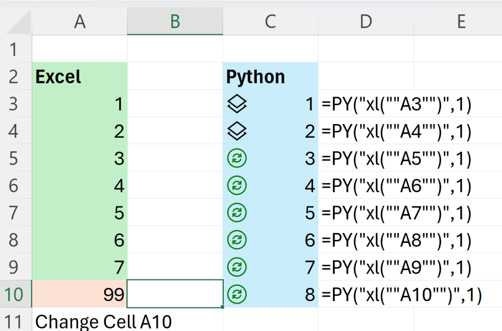
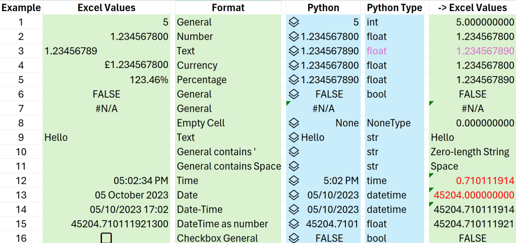
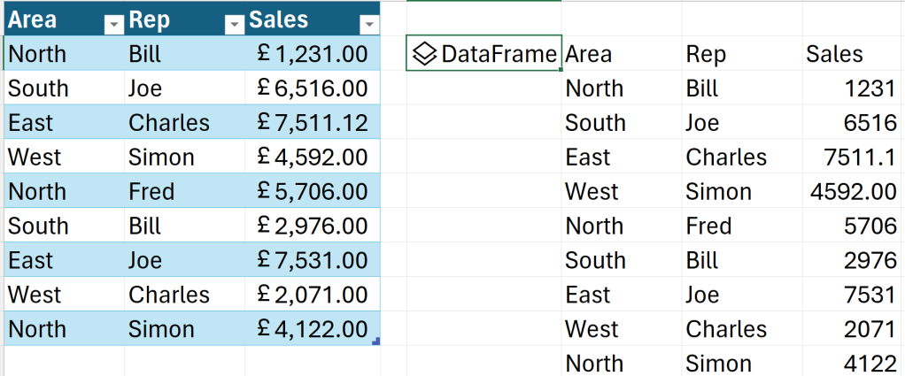
Manual Calculation No Longer Viral!

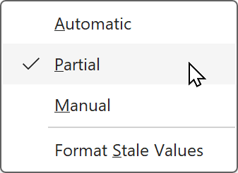
Excel has 3 basic calculation modes: Automatic, Manual and Automatic except Tables.

But an Excel session can currently only have one Calculation mode (unless you are using FastExcel which allows open workbooks and their worksheets to have different Calculation Modes).
Excel chooses the session calculation mode from the first workbook opened (the calculation mode is stored in every saved workbook).

Viral Manual Calculation Mode in previous Excel Versions

If the first (non-Addin) workbook you open was saved in Manual mode then the Excel session stays in Manual mode even when you open another workbook that was saved in Automatic mode (Of course you can change Excel’s calculation mode using the Ribbon or VBA).

In Excel versions before Office 365 or Excel 2021:

• Start Excel
• Open a Manual Workbook
• Open an Automatic workbook
• Save the Automatic Workbook
• Close Excel and then re-open the saved Automatic Workbook
• Excel is now in Manual Mode, the saved workbook has been changed to Manual!

If your users are in the habit of having multiple workbooks open at the same time and one of these workbooks is in Manual mode then Manual mode will soon spread virally to the other workbooks.

Excel 365 and Excel 2021

The change in Excel 365 and Excel 2021 is not to change the calculation mode of a workbook when saving it unless the user (or VBA) has changed Excel’s calculation mode before the save.

• Start Excel 365 or 2021
• Open a Manual Workbook
• Open an Automatic workbook
• Save the Automatic Workbook
• Close Excel and then re-open the saved Automatic Workbook
• Excel is now in Automatic Mode, the saved workbook has NOT been changed to Manual!

Advertisement

Only Calculating the Active Workbook

When you have more than one workbook open Excel has always recalculated all of the workbooks at each recalculation. That can be very painful if one or more of the workbooks are slow to calculate.

Now the Excel Dev Team has made a significant change to this process. When in Automatic calculation mode only the active workbook and any workbooks that it links to/from will be recalculated.

This change is currently only available to Insiders in the Beta channel running Windows version 2208 build 15529 or later and Mac version 16.64 build 22081401.

Testing Active Workbook Calc

I ran some tests using Insider Excel build 16224.20000.

Workbook 1 has a volatile formula =NOW() in D1 that shows when the formula was last calculated.

Workbook 2 has a formula in A2 =A1+1 and a volatile formula =NOW() in cell C1.

Both workbooks are visible in their separate windows.

With Workbook 2 active I changed cell A1 several times over the course of a few minutes and checked that the time shown in cell C1 changed – it did. But the time shown in Workbook 1 cell D1 did not change. And when I switched the active window to Workbook 1 then cell D1 did not change: just changing the active workbook does not trigger a recalc.

Next I added a FastExcel UDF CalcSeqCountRef(C1) to book 2 and CalcSeqCountRef(D1) to book 1. CalcSeqCountRef counts the number of times the referenced cell has been recalculated.

Now the time shown in book 1 always remains in sync with book2. This is because VBA UDFs are considered as workbook links to the workbook (in this case an XLAM addin) that contains the VBA code, so Excel considered Book1 and Book2 to be interlinked.
(By the way – UDFs in an XLL addin as opposed to an XLAM addin are not considered as links)

Exceptions to Active Workbook Calc

Active Workbook Only calc will not happen if:

• The workbook uses real-time streaming.
• Excel is in Manual Calc mode.
• You press F9 or Calculate Now.
• Your VBA triggers a recalculation.

Comparison with FastExcel Active Workbook Mode

For my FastExcel product I chose to focus more on Manual Calc mode, because when you have large slow workbooks you will tend to be using Manual.

FastExcel allows you to set Active Workbook Mode so that Excel will only calculate the active workbook.
When you set Active Workbook Mode the default is that each open workbook is in Manual calculation mode, so that you have to press F9 to calculate the Active Workbook but not any other workbooks.
(For more complicated situations FastExcel allows you to set different calculation modes for each open workbook.)

Conclusion

The beauty of the new Excel Active Workbook Calc is that it is automatic – you don’t have to do anything and it works well.
But the downside is that it does not work in Manual mode, which is arguably when you need it most!

Excel Screen-updating Performance Comparison.

The time that Excel takes to refresh the screen display can be a significant factor in overall processing speed.

Things that affect screen updating Time

• Excel only updates the visible part of the Excel windows – changing Zoom, the size of the visible window or changing to a different resolution monitor will change screen updating time.
• The more cells that change within the visible windows the slower screen updating will be. So switching to an empty worksheet minimises screen update time.
• Complexity of formatting – the more work Excel has to do to format visible cells the slower screen updating will be. Using heavy conditional formatting rules is the most severe cause of slow screen updating.
• Updating the statusbar – frequently updating statusbar text can be slow.

My benchmarking workbook

The workbook contains one sheet (Sheet1) with 4895 formulas and 1000 constants. Sheet2 and Sheet3 are empty. The workbook does not contain any Conditional Formatting or VBA.

You can down load the workbook from here

For Range Calculate timings select Sheet1!A1:BE89 and then View – Zoom to selection so that all the 5073 cells are visible.

Excel should be in Manual calculation mode.

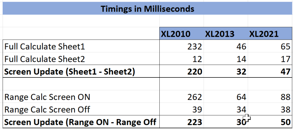
Screen Updating times for XL 2010, XL 2013, and XL 2021

Why are screen updating times so different by Excel Version? Some possible explanations:

In early versions of Excel parts of Excel’s rendering engine were coded in Assembler so as to maximise performance. As more function was built-in to the engine and Excel got supported on multiple end-points (Windows, IOS, Android) the use of Assembler became impractical and it became necessary to migrate as far as possible to a common cross-platform code-base.

But these changes had a drastic impact on screen-updating time, and the team decided that the only way to minimise this slow-down was to minimise the number of times the screen was updated. This turns out to be a complex task with potentially unfortunate side effects. Long-running tasks (calculation, VBA etc) running on the main Excel thread tended to show crazy looking or empty screens: Excel had cleared screen components but not yet redrawn them.

Excel 2010 has not fully implemented the minimisation of the number of screen redraws: screen update time is large.

Excel 2013 and 2021 have implemented minimising screen redraws.

I think Excel 2021 has fixes for some of the screen updating glitches, and also some features require additional work in the screen refresh, so 2021 is slightly slower than 2013.

Benchmarking screen updating time

I use 2 different methods to isolate and measure screen updating time. Both methods require the use of the Windows high-resolution timer. See https://fastexcel.wordpress.com/2011/05/31/a-quantum-of-time/

The Range Calculate method

The VBA Range Calculate method does a single threaded calculate of a range. If your VBA code switches ScreenUpdating to false then calls a timed Range.Calculate the time taken will exclude screen refresh time. Subtracting that from the Range Calculate time with ScreenUpdating true gives you screen refresh time. (Note you should be in Manual calculation mode. to avoid including the automatic recalc after Range Calculate).

First select and make visible the range of cells for which you want to measure screen update time then use the timed Range Calculate on the selection.

The CalculateFull method

The VBA Calculate Full method forces Excel to calculate every formula in the active workbooks.
Activate the worksheet that contains the formulas you want measure screen update time for. Use the high-resolution timer to measure the full calction, then switch to a completely empty sheet and repeat the Calculate Full timing. The difference between the 2 timings is the screen refresh time.

With this method you do not need to be in manual calculation mode or switch ScreenUpdating to False, but you need to do several successive full calculations to allow the multi-threaded recalc to self optimise.

Short-circuiting in Array Formulas

The previous post demonstrated that IF and CHOOSE short-circuit but IFS and SWITCH do not.

But following up a hint from Bill Wu that IF behaves differently in array formulas I decided to check whether it still short-circuits.
(IF in array formulas currently only returns a maximum of 255 characters but non-array IF does not have this limitation)

The short answer is that IF and CHOOSE do not short-circuit in array formulas but use a different and very efficient trick. So lets see how they work.

I am using the same VBA Pass UDF as in the previous post but using an array instead of a single value as the first argument to IF.

Option Explicit

Function Pass(valu As Variant)
    Pass = valu
    Debug.Print valu
End Function

The results in the immediate window are slightly surprising:

So what is Excel doing here?

The standard way Excel handles functions is to first evaluate each of the function arguments and only then call the function and pass it the results of the argument evaluations.
When the IF is an array function instead of doing short-circuiting it works in the standard non-short-circuiting way:

• B5:B8 evaluates to an array containing False, False, True, False
• Pass(80) evaluates to 80 and puts 80 in the Immediate window.
• Pass(90) evaluates to 90 and puts 90 in the Immediate window
• Then the IF function is called with these values.

Excel knows that it has to return 4 values so creates a 4 cell output array and then calls the IF function 4 times passing it a single value from the True/False array and the 80 and 90 result of evaluating the Pass functions. Excel puts the results of the 4 IF calls into the output array and finally returns the array to the grid. This array process is called “Lifting”

This lifting process is very efficient because the 2 Pass() arguments only get evaluated once rather than 4 times.

What about CHOOSE, IFS and SWITCH?

The same lifting process happens for array formulas of CHOOSE, IFS and SWITCH (and indeed all other functions that are not natively array capable).

255 character limit in Lifting?

I wonder if the reason for the 255 character limit is that Excel has to create the output array before calling the function so does not know what the maximum return size is, and for efficiency reasons creates fixed length array items which then get appropriately trimmed when returning to the grid.

Short-circuiting Excel Formulas: IF, CHOOSE, IFS and SWITCH

What is formula short-circuiting?

Short-circuiting occurs in Excel formulas when an IF statement only evaluates the True part of the IF and skips the False part of the IF. For example in this formula:

=IF(1>2,SUM(A10:B1000),SUM(C10:D1000))

Because 1>2 evaluates to False the SUM(A10:B1000) calculation never gets evaluated – only the SUM(C10:D1000) calculation is done.
Short-circuiting with IF is useful to avoid doing slow calculations when they are not needed and to avoid creating errors.

Which Excel functions short-circuit?

As of January 2023 there are 4 Excel conditional functions that could short-circuit:

• IF
• CHOOSE
• IFS
• SWITCH

But of these 4 only IF and CHOOSE actually short-circuit – IFS and SWITCH do not short-circuit. We can test this using a VBA UDF that tells us when it gets executed.

Option Explicit

Function Pass(valu As Variant)
    Pass = valu
    Debug.Print valu
End Function

Every time that the Pass function gets called it will write the valu variable to the VBE Immediate window (VBE – Ctrl G).
So now we can write formulas using IFS, IF, CHOOSE and SWITCH to see how they work.

Clicking Ctrl-Alt-F9 forces Excel ro recalculate all these formulas and the Pass UDF will output its results to the Immediate window.
The results appear in what looks like reverse sequence because Excel calculates formulas in last-entered first-calculated sequence (until the sequence is altered).

The IFS formula returns 3 to the grid, but shows 1 2 3 4 5 in the Immediate window – every component of the IFS formula has been executed – IFS does not short-circuit.

The IF formula returns 10 to the grid and only shows 10 in the Immediate Window – only the pass(10) has been executed – IF does short-circuit.

The CHOOSE formula returns 12 to the the grid and only shows 12 in the Immediate window – only the pass(12) part has been executed – CHOOSE does short-circuit.

The SWITCH formula returns 22 to the grid, but shows 21 22 23 in the Immediate window – ecery component of the SWITCH formula has been executed – SWITCH does not short-circuit.

Why do CHOOSE and IF short-circuit but IFS and SWITCH do not?

Normally the Excel formula interpreter evaluates all the arguments of a function before passing them to the function.

So in order to short-circuit IF and CHOOSE I think the Excel formula interpreter must recognise IF and CHOOSE as a special type of interpreter native function and evaluate the choice-of-arguments logic before evaluating the arguments in the usual left-to-right sequence.

Some people would regards the IFS and SWITCH behaviour as a bug!

Finding VBA Bottlenecks with VBA Profiler

When you are faced with slow-running or complex VBA projects it can be very helpful to have a tool that allows you to time the individual parts of your code or trace the execution path as event-driven jumps occur.

Googling for VBA profiler shows several VBA Profiling solutions, but none of them really did what I was looking for. So I decided to develop my own VBA Profiler – FastExcel ProfVBA.

Acknowledgements

I am very grateful to Stephen Bullen and Rob Bovey for their help in providing some of the initial code: see pages 546-500 of “Professional Excel Development” ISBN 0-321-50879-3.

And thanks also to Don Soloway for his collaboration on the project. In particular he developed the code for profiling loops and for showing results in the Immediate window.

ProfVBA Design Objectives

The things I wanted the Profiler to do were:

• Make Profiler commands available both from the Excel Ribbon and the VBE
• Easy to use ways of automatically inserting and removing Profiler calls to/from VBA
• One-click drill-downs into chosen VBA Procedures
• Work with VBA Userforms, Subs, Functions and Classes
• Do both Profiling and Tracing
• Start and stop Profiling
• Generate a Profiling report that prioritised the slow parts of the code.

Inserting Profiler Calls in your VBA

To time your VBA statements calls to ProfVBA need to be inserted into your code. Start and End calls should surround the block of code you want to time.

Usually you start by adding start and end calls to every sub and function in a project.
You could do this by manually inserting the calls, but this is difficult for VBA projects with many subs and function.

So ProfVBA uses the VBE Object Model to add the calls to your VBA source statements.
https://docs.microsoft.com/en-us/office/vba/language/reference/visual-basic-add-in-model/objects-visual-basic-add-in-model#codemodule

Adding start calls is easy but many subs/functions have multiple exit statements and so ProfVBA needs to identify all these.

Clicking “Add Profiler Calls” shows a Form so that you can choose where to add the calls.

ProfVBA has added a Start call at the beginning of the sub and End calls before both the Exit Sub and End Sub statements.

This statement in FastExcel ProfVBA inserts a start call after the current line in the body of your code module.

                'Insert a line for the ProfVBAProcStart call
490             oCM.InsertLines lBodyLine + 1, "gfxlProfVBA.ProfVBAProcStart """ & sProcID & """"

After adding the calls:

• Enable Profiling
• Run your VBA
• Show the Profiling Report

To profile a particular action from a userform, click the enable profiling button then click the button on the form and then view the profiling report.

The report shows which procedures are using the VBA execution time.

Exclusive or Inclusive Time

Exclusive time means that the timings shown are the times used by the procedure exclude the times used by child procedures called by the parent procedure.

You can choose either Exclusive or Inclusive timing in the Enable Profiling Options form:

Drilling Down into Your VBA

Once you have discovered which procedures are using the most execution time you can drill down to find out the most expensive blocks of statements.

You can use the ProfVBA VBE Toolbar to do this:

Select the Procedure in the VBE

Click the Insert Profiler Calls button

This will automatically use the selected Procedure.
Then you can choose one of the 3 drill-down methods

• Every Nth Line: this inserts Profiler start and end calls around every n lines of VBA code.
• All Loops in Proc: This inserts Profiler start and end calls around all the loops in the proc.
• Every Iteration of the Loops: this inserts Profiler start and end calls inside each loop in the proc and tracks each iteration of the loop separately.

Thanks to Don Soloway for implementing the Profiling Loops feature.

Summary

FastExcel ProfVBA provides easy-to-use methods of profiling your VBA code to find out where the VBA execution time is being used.

You can download a trial version of FastExcel from here.

http://www.decisionmodels.com/FastExcelV4_Install.htm

Excel Virtually Global

https://excelvirtuallyglobal.com/

Tue 21 July to Thu 23 July 2020

Microsoft’s Most Valuable Professionals, or MVPs, are technology experts
who passionately share their knowledge with the community. They are
always on the “bleeding edge” and have an unstoppable urge to get their
hands on new, exciting technologies. This virtual conference, now in its
fifth year, presents Excel, Data Platform and PowerPoint MVPs, together
with other acknowledged experts from Microsoft and / or around the globe
to present, answer questions and demonstrate the future of Excel and how
it will make your life easier, personally and professionally.
Topics include: Auditing Spreadsheets, Charts, Dashboards, Data
Analysis, Data Types, Dynamic Arrays, Excel Tricks & Tips, Financial
Modelling, Forecasting, Maps, Microsoft 365, New Functions and Features,
PivotTables, Power BI, Power Pivot, Power Query, Presenting Your Data,
Spilled Formulae, Testing, Timelines and developing solutions with DNA
.Net, VBA, Python, R, OfficeScript and Office-JS. And note well – it’s
not all in English, with sessions in Mandarin, Portuguese, Spanish and
Telugu, as well.

Most sessions will be recorded so you may watch them later with
downloads aplenty – there are no medals for staying up to watch the
entire event live!

From your own favourite chair, bring a laptop, an inquisitive mind and
your sense of humour. Be prepared to learn heaps. And remember, it’s
for charity – all profits will be donated to a global COVID-19 research
charity.

Price only US$23 Tickets at
https://www.eventbrite.com/e/excel-virtually-global-a-virtual-excel-summit-tickets-106319837496
(or just click ‘Register’ on the first site)

FastExcel Version 4 – with Introductory Offer

After several man-years of development and a lot of beta testing FastExcel Version 4 has finally hit general availability!

FastExcel V4 is a major rewrite of FastExcel V3 and provides many of the things you have been asking for:

• Support for the new capabilities and functions of Excel 2016, 2019 and Office 365 Excel
• 50 Powerful Dynamic Array Functions
• Formula Explorer for reviewing, undestanding and debugging formulas
• VBA Performance Profiling
• Single-click Drilldown to calculation bottleneck formulas
• Check Workbook for potential problems
• Choice of Automatic or Manual Install without Admin Privileges, uses .Net 4
• Separate Ribbon Tabs for Profiler, Manager Pro and SpeedTools
• Several hundred detailed improvements

Introductory offer: 40% Discount on FastExcel V4 Bundle and FastExcel Manager Pro for Mac!

Purchase FastExcel V4 Bundle using Coupon Code FXLV4INTRO – 40% Discount Offer valid until 15 April 2020.

Purchase FastExcel V4 Manager Pro for Mac using Coupon Code FXLMACINTRO – 40% Discount Offer valid until 15 April 2020.

FastExcel V4 Profiler Improvements

• • Single-Click Drill-Down Wizard: One click drill-down to the slowest formulas on the slowest worksheets

  • Improved Profiling Statistics: Counts of Unique Formulas, CSE Formulas and What-If Tables

  • Improved Profiling Stability

    • Changes in Excel memory managements made determining memory used by each worksheet both inaccurate and a cause of crashes. The measuring worksheet memory option has been removed.

  • Profile Formulas updated for new Excel and SpeedTools functions

  • VBA Performance Profiling

    • Choose VBA Project to Profile
    • Select Modules, Classes, Subroutines and Functions to Profile
    • Drill Down Profiling to blocks or single statements

  • New Check Workbook Report shows for each worksheet a range of statistics on potential workbook trouble spots.

    • Formulas: Counts of – Total Formulas, Unique Formulas, Error Formulas, CSE (Array) Formulas
    • Counts of Data Validation and Conditional Formats
    • Counts of What-If Tables, Table Onjects, Pivot Tables, Charts, Custom XML Parts, Shapes, Hyperlinks, Links, Defined Names
    • Used Range, Waste % and Sparse %

FastExcel V4 Manager Pro Improvements

• Manager Pro for Mac Excel 365

• New Formula Explorer Pro – A better way of reviewing, understanding and debugging formulas

  • Treeview of Formula Expressions
  • Normal, Precedent or Dependent Views
  • Forward and backward stepped debugging
  • Fully expanded Arrays expressions
  • Integrated understand of Excel functions like IF, SUMIFS, SUMPRODUCT etc
  • Work with Named Formulas, Conditional Format Formulas, Data Validation Formulas
  • Supports both US English and National Language formulas

• Name Manager Pro Improvements

  • Integration with Formula Explorer Pro: Review and Debug Named Formulas
  • Support of Office 365 Excel

• New Check Workbook Report

  • A report for each worksheet showing a range of statistics on potential workbook trouble spots.
    • Formulas: Counts of – Total Formulas, Unique Formulas, Error Formulas, CSE (Array) Formulas
    • Counts of Data Validation and Conditional Formats
    • Counts of What-If Tables, Table Onjects, Pivot Tables, Charts, Custom XML Parts, Shapes, Hyperlinks, Links, Defined Names
    • Used Range, Waste % and Sparse %

FastExcel V4 SpeedTools Improvements

• Easier formula entry with built-in Intellisense, Function Wizard and On-Line Help Support

• 100 super-fast powerful multi-threaded worksheet functions

  • Advanced FILTER.IFS, ASUMIFS family of functions
  • Logical AND, OR for array functions
  • Advanced AVLOOKUP and AMATCH functions

• Exploit the power of Dynamic Arrays with 50 Array-Handling functions

  • Totalling for Dynamic Arrays
    • Dynamically floating or static
    • Columns or Rows totals
  • Stack multiple Arrays/Ranges horizontally or vertically, handling headers
  • Unpivot using single or multiple headers and choice of columns
  • Merge (Join) dynamic arrays and find miss-matches (Anti-Join)
  • Resize & Reshape Arrays
  • Two-way Lookups and Slices
  • Multi-Column and Multi-row Lookups
  • Regular Expressions

Try it out for yourself:

Download FastExcel V4.

Get a 15-day full-featured trial license

You can convert the trial version of FastExcel V4 to a fully licensed version at any time by purchasing one of the FastExcel V4 licensing options.

Want to know more?

View the FastExcel V4 WebHelp

• FastExcel V4 Profiler WebHelp
• FastExcel V4 Manager Pro WebHelp
• FastExcel V4 SpeedTools WebHelp

Backward Compatibility of Office 365 Dynamic Arrays (Updated 23 Sep 2020)

Office 365 Excel Dynamic Arrays are great, but:

What happens when you create a workbook with Dynamic Array  Excel (Excel DA) and send it to someone who does not have Excel DA, and how do you write VBA code that works in both Excel DA and Excel Non-DA?

My free CheckDA tool allows you to check that the formulas you create using Excel DA will not cause problems when opened in prior Excel versions.

The introduction of Dynamic Array formulas in Office 365 Excel has made a fundamental change to Excel formula behavior and syntax:

• In previous versions such as Excel 2013, Excel automatically used implicit intersection to select a single value from a range in many circumstances.
• In Office 365 Dynamic Array Excel 2016 (Excel DA), Excel treats all formulas as array formulas unless the implicit intersection operator @ is used, and single-cell dynamic array formulas will spill their arrays to surrounding cells.

Forward Compatibility

For workbooks authored in previous versions of Excel compatibility is great: implicit intersections will be silently converted to the new @ syntax, and VBA code generally works fine.

Backward Compatibility

When workbooks authored in Dynamic Array Excel (Excel DA) are opened in previous Excel versions, in most cases the formulas will be silently converted to the old syntax (@ will be removed where possible, and spilling dynamic arrays converted to array (CSE) formulas).

Formulas created by VBA using Range.Formula will work correctly in both DA and non-DA Excel

But it is possible to create formulas in Excel DA which cause difficulties when opened in previous versions.

CheckDA is a free open-source VBA addin that can scan Excel DA formulas, highlight potential backward compatibility problems and optionally convert some problem formulas to more compatible versions.

Backward Compatibility Problem Areas

VBA code creating formulas

For forward compatibility reasons formulas created using Range.Formula are treated as old-style non-DA formulas. To create a DA formula using VBA you should use the new Range.Formula2.

Therefore if you want your VBA code to run in both DA and non-DA Excel use Range.Formula.
For more details see https://docs.microsoft.com/en-us/office/vba/excel/concepts/cells-and-ranges/range-formula-vs-formula2

VBA Object Model Extensions for Dynamic Arrays

In addition to .Formula2 the Excel team has added a few useful extensions to the VBA object model:

• Range.HasSpill returns True for both the parent DA formula and a spilled cell
• Range.SpillParent returns the Range object of the parent DA cell
• Range.SpillingToRange returns a range object covering the entire spill range
• Range.SavedAsArray returns true if the range will be converted to a CSE array formula in Non-DA Excel

Functions that do not exist in previous versions

Excel DA introduces many new functions that work with Dynamic Arrays (SORT, UNIQUE, LET …). When you open a workbook containing these functions in non-DA Excel:

• The cells will still show the values calculated in DA Excel, until they are recalculated.
• In Non-DA Excel the functions will be prefaced by xlfn. and as soon as you recalculate will show #Name.
• When the workbook is re-opened in DA Excel the xlfn. prefix is removed and the cells can be recalculated.

This means that limited DA<->NonDA round-tripping is possible even when these functions do not exist in NonDA!

Unexpected @ in a formula producing =_xlfn.SINGLE()

Excel will only remove @ from a formula where previous Excel versions would have used Implicit Intersection to return a single value from a Range or Named Range or function parameter.

You will be warned by Excel DA if you try to enter a formula with @ in an unexpected place, but it is still possible to create such a formula. An unexpected @ will create a _xlfn.SINGLE() in previous versions and will result in #Name when calculated.

For example =@A1 will be converted to =_xlfn.SINGLE(A1) because Excel cannot do Implicit Intersection on a single cell.

CheckDA will flag such formulas as type @

Formula containing a Spill Reference producing _xlfn_ANCHORARRAY()

A formula reference to a dynamic array can use the spill reference suffix #. For example =SUM($B$3#) will SUM the entire dynamic array that starts in $B$3. Spill references get converted to _xlfn_ANCHORARRAY(Reference) in previous versions and will result in #Name when calculated.

CheckDA will flag such formulas as type {#}

Unwanted Array Formulas (CSE) in previous versions

Any formula that Excel DA thinks could return an array (even if it is actually only returning a single value) is converted to a CSE array formula in previous versions.

This may or may not produce a backward compatibility problem – you have to inspect these formulas carefully.

CheckDA flags these formulas as types:

• {1} a single-cell non-spilling formula
• # An Excel DA Dynamic Array formula that is spilling or blocked (#Spill!)  will be converted to a fixed CSE formula in previous Non-DA Excel versions such as Excel 2013.
• {n} a formula entered in Excel DA as a multi-cell CSE formula

Using CheckDA

CheckDA is an open-source VBA XLAM addin.
CheckDA only runs in Windows Office 365 Dynamic Array Excel.

To protect against accidental change CheckDA is protected with the password dm.

You can download the CheckDA addin from here. The zip file contains the CheckDA.xlam and the CheckDa.docx Word document.

Install the CheckDA.XLAM file using Excel’s Addin Manager if you want it permanently installed, or just open the xlam workbook using Excel File Open if you only want to use it in the current Excel session. Once successfully installed you will see CheckDA available on the ribbon.

Control-Shift-J or clicking the Check DA Formulas button shows the Check DA form.

The form:

• Shows formulas in Non-DA Syntax
• Is Modeless (you can edit formulas while still showing the form)
• Is Resizeable
• At start-up scans the active worksheet for unique formulas
• At start-up filters out formulas with unexpected @ or Spill Ref or Spill or single-cell array formulas

Restate Selected Formulas

Clicking the Restate Selected Formulas button will change any @ or {1} formulas selected in the form to more compatible syntax:

• @ formulas will have their unexpected @s removed.
• {1} formulas will be re-entered as non-array formulas.
• # Spill formulas and {#} Spill Ref formulas cannot be automatically restated.

Undo Restate

Clicking the Undo Restate button will undo the restatement of any formulas restated in this session of CheckDA.

Show Office 365 DA Syntax

This button toggles between showing the formulas in Non-DA syntax and Office 365 Dynamic Array syntax.

Conclusion

The Microsoft Excel team have done an outstanding job of creating, as far as is possible, compatibility between Dynamic Array Excel and previous versions. With a little care you can easily create workbooks using Excel DA that work correctly in Non-DA Excel.

Further Reading

• the spilled range operator and how to use it
• the various dynamic array behaviors
• how dynamic arrays compare to legacy array formulas
• new #SPILL error and scenarios that can trigger it
• implicit intersection and dynamic arrays
• dynamic arrays in prior versions of Excel
• Range.Formula2 https://docs.microsoft.com/en-us/office/vba/api/excel.range.formula2
• Range.Formula vs Range.Formula2: https://docs.microsoft.com/en-us/office/vba/excel/concepts/cells-and-ranges/range-formula-vs-formula2

Excel Summit South 2019

If you can get to Australia in July/August check out the Excel Summit South 2019 conference.

http://excelsummitsouth.com/

There is a great list of speakers and a chance to discuss Excel with a Microsoft Dev Team member and a host of Microsoft Excel MVP’s – acknowledged as Experts and Community contributors by Microsoft.